[Machine Learning] PyTorch로 선형 회귀 구현하기 (Linear Regression)

PyTorch을 사용해 선형 회귀(Linear Regression)을 구현해보자.

먼저 PyTorch의 설치는 이전 포스팅을 참고하자.

[PyTorch] m1 맥에 GPU 사용 Pytorch 설치 및 에러 해결 / ERROR: Could not find a version that satisfies the requirement torch

---

먼저 필요한 라이브러리를 임포트하자.

import torch
import matplotlib.pyplot as plt

 

이제 임의의 데이터셋을 만들어보자.

x = torch.rand(100)
# Calculate y = 3x + 2 + epsilon
y = 3*x + 2 + torch.rand(len(X))

먼저 x는 100개의 0부터 1까지의 랜덤 넘버이고 y는 x에 3을 곱한 다음 2를 더한 것에 오차를 준 것이다.

이해가 잘 가지 않는다면 꼭 x와 y을 출력해서 데이터셋을 이해하고 넘어가자.

참고로 100개의 데이터 (x, y)을 점으로 찍어볼 수도 있다.

plt.scatter(x, y)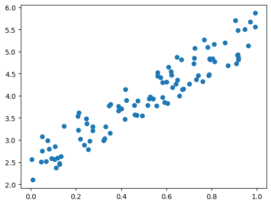

scattering plot of (x, y)

선형 회귀는 데이터를 대표할만한 직선을 찾는 것이다.

따라서 선형 회귀의 목표는 위의 플랏에 데이터의 분포와 가장 잘 맞는 직선 \( y = W\times x + b \)을 찾는 것이다.

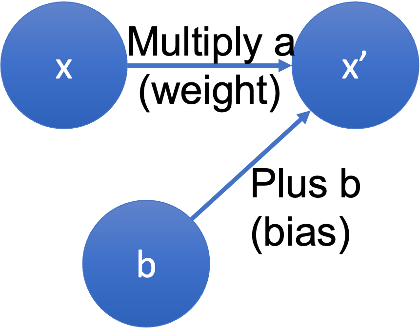
아래와 같은 Hypothesis(가설)을 세우자. $$ y = W\times x + b $$

이제 우리가 찾아야할 값은 \(W\)와 \(b\)이다.

이를 코드로 써보면 아래와 같다.

W = torch.rand(1, requires_grad=True)
b = torch.rand(1, requires_grad=True)
hypothesis = W * x + b

이때 requires_grad=True는 트레이닝을 통해 값이 변경되는 모델의 매개 변수라는 것을 뜻한다.

위의 코드에서 W와 b을 랜덤 넘버로 설정해였기 때문에 현재 직선은 모델과는 거리가 멀다.

참고로 값은 각각 0.2629, 0.5405이다.

plt.scatter(x, y)
plt.plot([0, 1], [(W.detach()*a+b.detach()) for a in [0, 1]], 'C1')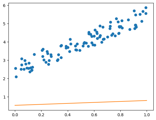

트레이닝 전 hypothesis

이때 .detach()는 연산 기록으로부터 변수를 떼어놓는 것이다.

 

이제 훈련을 위해 비용 함수를 설정하자.

비용 함수는 평균 제곱 오차(mse, mean square error)로 설정하였다.

cost = torch.mean((hypothesis - y)**2)

 

이제 optimizer도 설정하자.

optimizer는 SGD, 학습률은 0.01으로 설정하였다.

optimizer = torch.optim.SGD([W, b], lr=0.01)

 

이제 트레이닝하는 코드를 짜보자.

Epoch는 3000번으로 하였다.

nb_epochs = 3000 # 3000 epoch
for epoch in range(1, nb_epochs+1):

    hypothesis = W*x + b                      # Calculate H(x)

    cost = torch.mean((hypothesis - y) ** 2)  # Calculate cost

    # update H(x)
    optimizer.zero_grad()
    cost.backward()
    optimizer.step()

    if epoch % 100 == 0:
        print('Epoch {:4d}/{} W: {:.3f}, b: {:.3f} Cost: {:.4f}'.format(
            epoch, nb_epochs, W.item(), b.item(), cost.item()
        ))

 

이제 훈련이 완료되었으니 결과를 살펴보자.

plt.scatter(x, y)
plt.plot([0, 1], [(W.detach()*a+b.detach()) for a in [0, 1]], 'C1')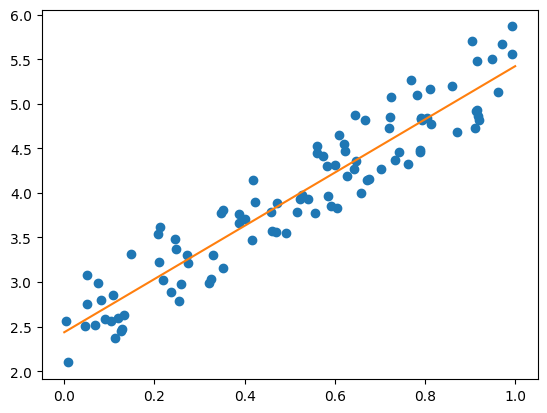

트레이닝 후 hypothesis

직선과 데이터가 잘 맞는 것을 확인할 수 있다.

이제 우리가 세운 hypothesis(가설) \( y = W\times x + b \)이 데이터를 대표한다고 말할 수 있을 것이다.

참고로 W와 b을 출력해보면 각각 2.9845, 2.4361값이 나온다.

우리가 데이터를 만들 때 y=3x+2의 관계를 가지도록 설정했기 때문에 b의 값이 의아할 수 있다.

우리가 앞에서 설정한 b의 값의 차이 즉, 약 0.5는 노이즈를 더한 것에서 기인한 것으로, 3x+2에서 0에서 1 사이의 랜덤 넘버를 더했기 때문에 훈련된 값도 노이즈의 평균인 0.5정도가 더해진 채로 훈련된 것이다.

 

전체 코드는 다음과 같다. 플랏을 저장하는 코드가 없으니 주피터 노트북이나 주피터 랩에서 돌려보자.

import torch
import matplotlib.pyplot as plt

x = torch.rand(100)
# Calculate y = 3x + 2 + epsilon
y = 3*x + 2 + torch.rand(len(X))
# plt.scatter(x, y)

W = torch.rand(1, requires_grad=True)
b = torch.rand(1, requires_grad=True)

# plt.scatter(x, y)
# plt.plot([0, 1], [(W.detach().numpy()*a+b.detach().numpy()) for a in [0, 1]], 'C1')

hypothesis = W * x + b

cost = torch.mean((hypothesis - y)**2)

epochs = 3000 # epoch 설정
for epoch in range(1, epochs+1):

    hypothesis = x * W + b # Calculate H(x)

    cost = torch.mean((hypothesis - y) ** 2) # Calculate cost

    # update H(x)
    optimizer.zero_grad()  # gradient을 초기화
    cost.backward()        # gradinet 계산
    optimizer.step()       # optimizer(즉, W와 b) 업데이트

    if epoch % 100 == 0:
        print('Epoch {:4d}/{} W: {:.3f}, b: {:.3f} Cost: {:.4f}'.format(
            epoch, nb_epochs, W.item(), b.item(), cost.item()
        ))
        
# plt.scatter(x, y)
# plt.plot([0, 1], [(W.detach()*a+b.detach()) for a in [0, 1]], 'C1')

print(W, b)

---

class을 사용해서 Linear Regression 구현하기

위와 동일한 데이터, 동일한 hypothesis을 가지고 모델을 클래스로 구현해서 트레이닝 해보자.

그리고 비용 함수도 PyTorch에서 제공하는 것을 사용해보자.

모델을 먼저 써보면 아래와 같다.

class LinearRegression(nn.Module):
    def __init__(self):
        super().__init__()
        self.linear = nn.Linear(in_features=1, out_features=1, bias=True)
	# torch.nn.Linear(in_features, out_features, bias=True, device=None, dtype=None)

    def forward(self, x):
        return self.linear(x)

nn.Linear을 사용하는데 보통 뉴럴 네트워크를 구성하는 아주 기본적인 단위가 되는 함수이다.

self.linear에서 bias가 True이므로

저 모델의 입력단과 출력단은 \(x -> ax\)에 바이어스 \(b\)가 포함된 \( x -> ax+b \)가 된다.

nn.Linear(1, 1, bias=True)

함수의 자세한 내용은 구글링을 하면 PyTorch의 공식 문서 링크가 나온다.

 

비용함수는 아래와 같이 쓰면 된다.

loss = torch.nn.MSELoss()

참고로 아래와 같이 사용할 수 있다.

loss = nn.MSELoss()
input = torch.randn(3, 5, requires_grad=True)
target = torch.randn(3, 5)
output = loss(input, target) # 단순히 x와 타겟(우리는 y)을 넣으면 계산을 해준다.
output.backward()

 

Optimizer에는 모델의 파라미터를 입력해야하는데 아래와 같이 클래스로 된 모델의 파라미터를 넣을 수 있다.

optimizer = torch.optim.SGD(model.parameters(), lr=0.01)

 

이제 모든 준비는 끝났으니 코드를 작성해보자.

이제는 torch.nn도 임포트를 해야한다.

전체 코드는 아래와 같다.

import torch
import torch.nn as nn
import matplotlib.pyplot as plt

x = torch.rand(100)
# Calculate y = 3x + 2 + epsilon
y = 3*x + 2 + torch.rand(len(x))
# plt.scatter(x, y)

class LinearRegression(nn.Module):
    def __init__(self):
        super().__init__()
        self.linear = nn.Linear(1, 1)

    def forward(self, x):
        return self.linear(x)

model = LinearRegression()
optimizer = torch.optim.SGD(model.parameters(), lr=0.01) 
loss = torch.nn.MSELoss()

# 주석을 해제하여 트레이닝 전 모델의 입출력을 확인해보자.
# plt.scatter(x, y)
# plt.plot([0, 1], [(model.get_parameter('linear.weight').detach()*a+model.get_parameter('linear.bias').detach()) for a in [0, 1]], 'C1')

# 모델의 입출력에 맞게 데이터의 맨 앞에 1차원 추가
x = x.reshape(-1, 1)
y = y.reshape(-1, 1)

epochs = 3000
for epoch in range(1, epochs+1):
            
    prediction = model(x)
    cost = loss(prediction, y)

    optimizer.zero_grad()
    cost.backward()
    optimizer.step()

    if epoch % 100 == 0:
        print('Epoch {:4d}/{} Cost: {:.4f}'.format(
            epoch, nb_epochs, cost.item()
        ))

# 주석을 해제하여 트레이닝 후 모델의 입출력을 확인해보자.
# plt.scatter(x, y)
# plt.plot([0, 1], [(model.get_parameter('linear.weight').detach()*a+model.get_parameter('linear.bias').detach()) for a in [0, 1]], 'C1')

주석으로 모델의 트레이닝 전후 입출력을 눈으로 확인할 수 있는 코드를 달아두었으니 확인해보자.

---

아주 아주 기본적인 머신 러닝 방법을 알아보았다.

다음엔 분류(classification)을 알아보도록 하자.