
저번 포스팅에서 모델 일반화(generalization)의 필요성과 일반화 중 어떤 방법이 있는지를 살펴보았다.
[Machine Learning] 오버피팅(Overfitting), 언더피팅(Underfitting)의 개념 및 해결 방법
위 글에서 오버피팅을 막기 위한 여러가지 방법을 소개했었다.
개념은 이미 설명했으니 헷갈리기 쉬운 개념 하나만 짚은 다음 그 방법들이 얼마나 효과적인지 직접 테스트 해보자.
Generalization와 Regularization의 차이점
일반화(generalization)와 정규화(regularization)는 서로 연관되어 있지만 별개의 개념이다.
일반화는 훈련된 모델이 본 적이 없는 데이터, 즉 훈련 중에 사용되지 않은 데이터(예를 들어, 테스트 데이터)에 대해 모델의 기능을 잘 수행할 수 있는 능력을 의미한다.
즉, 일반화를 잘 할 수 있는 모델은 새롭고 다양한 데이터 세트에 대해 정확한 예측을 할 수 있다.
반면 정규화는 보통 오버피팅 즉, 모델이 일반화가 되지 않고 훈련 데이터 세트를 과하게 학습하는 것을 방지하기 위해 트레이닝 중 사용되는 기술이다.
오버피팅은 모델이 너무 복잡하거나 일반화가 아닌 훈련 데이터를 모델이 암기하기 시작할 때 발생한다.
요약하면 일반화(generalization)와 정규화(regularization)는 서로 연관있는 개념이지만, 일반화는 모델이 처음 보는 데이터에 대한 성능을 뜻하는 반면, 정규화는 오버피팅을 방지하여 일반화 성능을 개선하기 위해 모델 훈련 중에 사용되는 기술이라고 볼 수 있다.
실험 방법
이제 "기술"에 해당하는 정규화(regularization)를 직접 테스트 해보자.
방법은 CIFAR100 데이터셋에 대해 모델을 트레이닝 하는데, 매 에포크마다 테스트 데이터에 대한 비용함수의 값을 출력할 것이다.
훈련이 진행됨에 따라 이 값은 감소하다가 오버피팅이 일어나면 값이 다시 증가할 것이다.
테스트 데이터에 대한 비용함수의 값이 낮아질 때마다 모델을 저장할 것이고 높아지면 모델을 저장하지 않고 계속 훈련할 것이다.
20 에포크 이상 테스트 데이터에 대한 비용함수의 값이 낮아지지 않는다면 오버피팅이 일어나는 것으로 간주하고 마지막으로 저장된 비용함수의 값으로 정규화(regularization)의 여러 방법에 대한 평가를 할 것이다.
염두에 둘 점은 어떤 정규화 기술이 가장 좋은지 겨뤄보자가 아니라 단지 방법을 소개하고 직접 돌려보는 것에 초점을 맞추는 것이다.
그냥 아무런 기술이 들어가지 않은 모델 (기준)
직접 모델을 만들어서 돌려보자.
먼저 사용할 데이터 세트를 다운로드하고 잘 다운로드 되었는지 확인해보자.
import torch as th
import torchvision as tv
from collections import defaultdict

trans = tv.transforms.ToTensor()
train = tv.datasets.CIFAR100('data/torchvision/CIFAR100', train=True, download=True, transform=trans)
test = tv.datasets.CIFAR100('data/torchvision/CIFAR100', train=False, download=True, transform=trans) # /data/torchvision
print(train, "\n", test)

trainloader = th.utils.data.DataLoader(train, batch_size=128)
testloader = th.utils.data.DataLoader(test, batch_size=128)

for images, labels in testloader:
    print(images.shape, labels.shape)
break아주 만약 여기서 URLError: <urlopen error [SSL: CERTIFICATE_VERIFY_FAILED] certificate verify failed: unable to get local issuer certificate이런 에러가 발생한다면 아래 코드를 먼저 실행해주고 다운로드하자.
import ssl
ssl._create_default_https_context = ssl._create_unverified_context아무튼 잘 실행이 된다면 아래와 같은 출력이 나올 것이다.
Dataset CIFAR100
    Number of datapoints: 50000
    Root location: data/torchvision/CIFAR100
    Split: Train
    StandardTransform
Transform: ToTensor()
 Dataset CIFAR100
    Number of datapoints: 10000
    Root location: data/torchvision/CIFAR100
    Split: Test
    StandardTransform
Transform: ToTensor()
torch.Size([128, 3, 32, 32]) torch.Size([128])이제 학습에 사용할 디바이스를 선택하자.
알아서 사용가능한 디바이스를 컴퓨터가 선택할 것이다.
device = th.device('cuda' if torch.cuda.is_available() else 'mps' if torch.backends.mps.is_available() else 'cpu') # For m1 Mac Users이제 모델을 만들자.
import torch.nn as nn

class Net(nn.Module):
    def __init__(self):
        super(Net, self).__init__()

        self.conv1 = nn.Sequential(
            nn.Conv2d(3, 6, 4, 2, 1, bias=False),
            nn.LeakyReLU(0.2, inplace=True))

        self.conv2 = nn.Sequential(
            nn.Conv2d(6, 12, 4, 2, 1, bias=False),
            nn.LeakyReLU(0.2, inplace=True))

        self.conv3 = nn.Sequential(
            nn.Conv2d(12, 24, 4, 2, 1, bias=False),
            nn.LeakyReLU(0.2, inplace=True))

        self.lin = nn.Sequential(
            nn.Linear(24*4*4, 100),
            nn.Sigmoid())

    def forward(self, input):
        conv1 = self.conv1(input)
        conv2 = self.conv2(conv1)
        conv3 = self.conv3(conv2)
        output  = self.lin(conv3.view(-1, 24*4*4))
return output이제 모델을 트레이닝하면서 트레이닝과 테스트 데이터 세트에 대한 비용함수를 계속 저장하자.
그리고 위에서 말했던 것처럼 연속으로 20 에포크 이상 테스트 데이터의 비용함수가 줄어들지 않으면 학습을 중단하고 테스트 데이터 비용함수가 가장 낮았던 모델을 세이브하도록 하자.
그리고 저장한 각각의 비용함수 값을 그래프로 그려서 어떻게 훈련이 진행되었는지 확인해보자.
(이번 글은 새로운 방법을 소개하는 포스팅이 아니고 단순 비교가 목적인 포스팅이라 코드가 다소 중구난방이지만 에러는 없다.)
참고로 오늘 돌릴 코드들은 시간이 좀 걸린다.
net = Net()
net.to(device)
opt = th.optim.Adam(net.parameters())
l = th.nn.CrossEntropyLoss()
per_epoch = defaultdict(lambda:[])
last_save = 0
e = 0

while last_save < 20:
# for i in range(20): # 20 epochs
    per_batch = defaultdict(lambda:[])
    net.train()
    for images, labels in trainloader:
        opt.zero_grad()
        outputs = net(images.to(device))
        loss = l(outputs, labels.to(device))
        loss.backward()
        opt.step()
        per_batch["loss"].append(loss.item()*images.size(0))
        per_batch["corr"].append(sum(th.max(outputs,1)[1].cpu()==labels))
        per_batch["n"].append(images.size(0))
    per_epoch["loss"].append(sum(per_batch["loss"])/sum(per_batch["n"]))
    per_epoch["acc"].append(sum(per_batch["corr"])/sum(per_batch["n"]))
    net.eval()
    with th.no_grad():
        for images, labels in testloader:
            outputs = net(images.to(device))
            loss = l(outputs, labels.to(device))
            per_batch["tloss"].append(loss.item()*images.size(0))
            per_batch["tcorr"].append(sum(th.max(outputs,1)[1].cpu()==labels))
            per_batch["tn"].append(images.size(0))
    per_epoch["tloss"].append(sum(per_batch["tloss"])/sum(per_batch["tn"]))
    per_epoch["tacc"].append(sum(per_batch["tcorr"])/sum(per_batch["tn"]))
    print(f'epoch {e:03d} : train loss {per_epoch["loss"][-1]:.3f} acc {per_epoch["acc"][-1]:.3f} test loss {per_epoch["tloss"][-1]:.3f} acc {per_epoch["tacc"][-1]:.3f}')
    # early stopping: if we are at the best epoch (= epoch with lowest loss), save the weights
    last_save += 1; e += 1
    if per_epoch["tloss"][-1] == min(per_epoch["tloss"]):
        print("  saving network")
        th.save(net.state_dict(), 'noRegularization.pt')
        last_save = 0
print("done training.")
# reload the best weights
net.load_state_dict(th.load('NoRegularization.pt'))
# Make plots of the training/testing losses
plt.plot(per_epoch["loss"], label="train")
plt.plot(per_epoch["tloss"], label="test")
plt.legend(loc="upper right")코드의 실행 결과는 다를 수 있는데 가장 낮았던 테스트의 비용함수와 내 결과의 마지막 줄, 및 그래프는 이렇다.
epoch 048 : train loss 3.973 acc 0.118 test loss 4.119 acc 0.095
  saving network

...

epoch 068 : train loss 3.960 acc 0.119 test loss 4.123 acc 0.096
done training.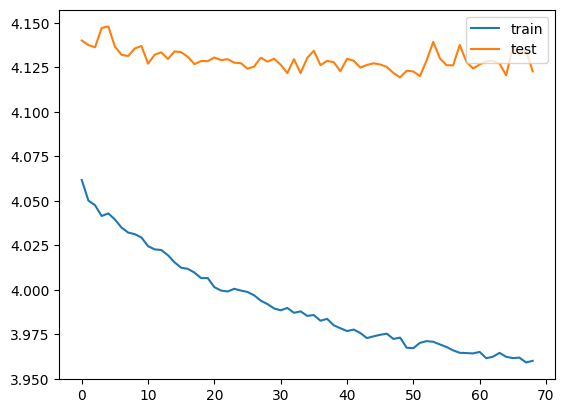
Weight Decay / 가중치 감쇠
Weight decay는 비용 함수에 패널티를 추가해서 가중치를 0에 가깝게 유지하는 것이다.
코드에서 optim = torch.optim.SGD(..., weight_decay=0.01)와 같은 방식으로 가중치 감쇠를 줄 수 있다.
이제 모델을 다시 선언하고 가중치 감쇠를 적용시켜 훈련을 진행한 다음 결과를 비교해보자.
net = Net()
net.to(device)
opt = th.optim.Adam(net.parameters(), weight_decay=0.001)
l = th.nn.CrossEntropyLoss()
per_epoch_with_weight_decay = defaultdict(lambda:[])
last_save = 0
e = 0

while last_save < 20:
# for i in range(20): # 20 epochs
    per_batch = defaultdict(lambda:[])
    net.train()
    for images, labels in trainloader:
        opt.zero_grad()
        outputs = net(images.to(device))
        loss = l(outputs, labels.to(device))
        loss.backward()
        opt.step()
        per_batch["loss"].append(loss.item()*images.size(0))
        per_batch["corr"].append(sum(th.max(outputs,1)[1].cpu()==labels))
        per_batch["n"].append(images.size(0))
    per_epoch_with_weight_decay["loss"].append(sum(per_batch["loss"])/sum(per_batch["n"]))
    per_epoch_with_weight_decay["acc"].append(sum(per_batch["corr"])/sum(per_batch["n"]))
    net.eval()
    with th.no_grad():
        for images, labels in testloader:
            outputs = net(images.to(device))
            loss = l(outputs, labels.to(device))
            per_batch["tloss"].append(loss.item()*images.size(0))
            per_batch["tcorr"].append(sum(th.max(outputs,1)[1].cpu()==labels))
            per_batch["tn"].append(images.size(0))
    per_epoch_with_weight_decay["tloss"].append(sum(per_batch["tloss"])/sum(per_batch["tn"]))
    per_epoch_with_weight_decay["tacc"].append(sum(per_batch["tcorr"])/sum(per_batch["tn"]))
    print(f'epoch {e:03d} : train loss {per_epoch_with_weight_decay["loss"][-1]:.3f} acc {per_epoch_with_weight_decay["acc"][-1]:.3f} test loss {per_epoch_with_weight_decay["tloss"][-1]:.3f} acc {per_epoch_with_weight_decay["tacc"][-1]:.3f}')
    # early stopping: if we are at the best epoch (= epoch with lowest loss), save the weights
    last_save += 1; e += 1
    if per_epoch_with_weight_decay["tloss"][-1] == min(per_epoch_with_weight_decay["tloss"]):
        print("  saving network")
        th.save(net.state_dict(), 'weightDecay.pt')
        last_save = 0
print("done training.")
# reload the best weights
net.load_state_dict(th.load('weightDecay.pt'))
# Make plots of the training/testing losses
plt.plot(per_epoch["loss"], label="train")
plt.plot(per_epoch["tloss"], label="test")
plt.plot(per_epoch_with_weight_decay["loss"], label="weight decay train")
plt.plot(per_epoch_with_weight_decay["tloss"], label="weight decay test")
plt.legend(loc="upper right")가장 낮았던 테스트의 비용함수와 결과의 마지막 줄, 그래프는 다음과 같았다.
epoch 054 : train loss 4.020 acc 0.155 test loss 4.115 acc 0.152
  saving network

...

epoch 074 : train loss 4.005 acc 0.162 test loss 4.119 acc 0.160
done training.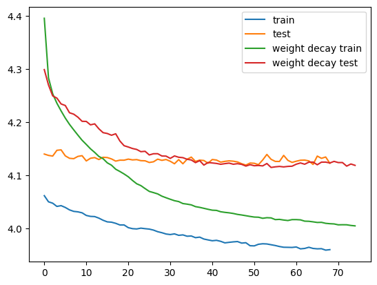
가중치 감쇠를 적용한 결과 비용함수의 값이 4.119에서 4.103으로 줄긴 했지만 드라마틱한 결과의 발전은 없었다.
사실 가중치 감쇠를 적용하면 학습률과 같은 파라미터도 손을 봐야하지만 비교를 위해(귀찮아서) 건드리지 않았을 뿐이다.
이 방법이 별로다라는 이야기는 결코 아니다.
Dropout
드랍아웃은 훈련 중에 일부 노드의 출력을 사용하지 않는 것으로 여러 모델을 앙상블한 효과를 준다.
어떤 텐서를 드랍아웃시키면 출력에 0이 나온다.
아래 코드로 확인해보자.
import torch
dropout = torch.nn.Dropout(0.5) # Creates the layer
x = torch.randn((6))
print("Initial:", x)
print("Dropout:", dropout(x)) # Use the layer얘를 돌리면 아래와 같은 결과가 나온다. (숫자나 0의 위치는 다를 수 있다.)
Initial: tensor([-0.8932, -0.8693, -0.6018,  1.4749, -0.2535,  1.6248])
Dropout: tensor([-1.7865, -0.0000, -1.2037,  0.0000, -0.5070,  0.0000])
이제 드랍아웃을 모델에 적용시키자.
이번에는 모델을 수정해야한다.
class Net(nn.Module):
    def __init__(self):
        super(Net, self).__init__()

        self.conv1 = nn.Sequential(
            nn.Conv2d(3, 6, 4, 2, 1, bias=False),
            nn.LeakyReLU(0.2, inplace=True),
            nn.Dropout(0.5, inplace=False))

        self.conv2 = nn.Sequential(
            nn.Conv2d(6, 12, 4, 2, 1, bias=False),
            nn.LeakyReLU(0.2, inplace=True),
            nn.Dropout(0.5, inplace=False))

        self.conv3 = nn.Sequential(
            nn.Conv2d(12, 24, 4, 2, 1, bias=False),
            nn.LeakyReLU(0.2, inplace=True),
            nn.Dropout(0.5, inplace=False))

        self.lin = nn.Sequential(
            nn.Linear(24*4*4, 100),
            nn.Sigmoid())

    def forward(self, input):
        conv1 = self.conv1(input)
        conv2 = self.conv2(conv1)
        conv3 = self.conv3(conv2)
        output  = self.lin(conv3.view(-1, 24*4*4))
return output다른 것은 건드리지 않고 드랍아웃만 추가했다.
이제 훈련을 시킨 다음 결과를 비교해보자.
net = Net()
net.to(device)
opt = th.optim.Adam(net.parameters())
l = th.nn.CrossEntropyLoss()
per_epoch_with_dropout = defaultdict(lambda:[])
last_save = 0
e = 0

while last_save < 20:
# for i in range(20): # 20 epochs
    per_batch = defaultdict(lambda:[])
    net.train()
    for images, labels in trainloader:
        opt.zero_grad()
        outputs = net(images.to(device))
        loss = l(outputs, labels.to(device))
        loss.backward()
        opt.step()
        per_batch["loss"].append(loss.item()*images.size(0))
        per_batch["corr"].append(sum(th.max(outputs,1)[1].cpu()==labels))
        per_batch["n"].append(images.size(0))
    per_epoch_with_dropout["loss"].append(sum(per_batch["loss"])/sum(per_batch["n"]))
    per_epoch_with_dropout["acc"].append(sum(per_batch["corr"])/sum(per_batch["n"]))
    net.eval()
    with th.no_grad():
        for images, labels in testloader:
            outputs = net(images.to(device))
            loss = l(outputs, labels.to(device))
            per_batch["tloss"].append(loss.item()*images.size(0))
            per_batch["tcorr"].append(sum(th.max(outputs,1)[1].cpu()==labels))
            per_batch["tn"].append(images.size(0))
    per_epoch_with_dropout["tloss"].append(sum(per_batch["tloss"])/sum(per_batch["tn"]))
    per_epoch_with_dropout["tacc"].append(sum(per_batch["tcorr"])/sum(per_batch["tn"]))
    print(f'epoch {e:03d} : train loss {per_epoch_with_dropout["loss"][-1]:.3f} acc {per_epoch_with_dropout["acc"][-1]:.3f} test loss {per_epoch_with_dropout["tloss"][-1]:.3f} acc {per_epoch_with_dropout["tacc"][-1]:.3f}')
    # early stopping: if we are at the best epoch (= epoch with lowest loss), save the weights
    last_save += 1; e += 1
    if per_epoch_with_dropout["tloss"][-1] == min(per_epoch_with_dropout["tloss"]):
        print("  saving network")
        th.save(net.state_dict(), 'dropout.pt')
        last_save = 0
print("done training.")
# reload the best weights
net.load_state_dict(th.load('dropout.pt'))
# Make plots of the training/testing losses
plt.plot(per_epoch["loss"], label="train")
plt.plot(per_epoch["tloss"], label="test")
plt.plot(per_epoch_with_dropout["loss"], label="dropout train")
plt.plot(per_epoch_with_dropout["tloss"], label="dropout test")
plt.legend(loc="upper right")결과는 아래와 같다.
epoch 172 : train loss 4.133 acc 0.100 test loss 4.088 acc 0.138
  saving network

...

epoch 192 : train loss 4.132 acc 0.101 test loss 4.095 acc 0.126
done training.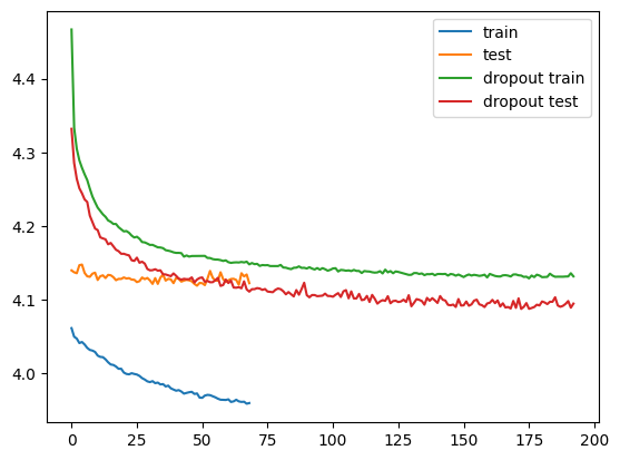
드랍아웃을 사용했을 때, 테스트 값이 기준인 4.119에서 4.090으로 조금 더 줄었다.
지금은 비교를 위해서 다른 조건을 건드리지 않았지만 드랍아웃도 가중치 감쇠와 마찬가지로 다른 파라미터들을 조정해가며 학습을 진행해야한다. (사실 모든 방법이 다 그렇다.)
BatchNorm
BatchNorm(배치 정규화)는 각 레이어의 입력을 정규화해서 평균이 0, 분산이 1이 되도록 하는 기술이다.
이렇게 하면 vanishing gradient(기울기 소실)을 방지하고 모델을 더 빠르고 정확하게 학습할 수 있어 아주 널리 사용되는 방법이다.
코드도 레이어의 출력 노드 수에 함수를 씌우면 된다.
...
nn.Conv2d(3, 6, 4, 2, 1),
nn.BatchNorm2d(6),
...이제 모델을 만들고 훈련을 시켜보자.
class Net(nn.Module):
    def __init__(self):
        super(Net, self).__init__()

        self.conv1 = nn.Sequential(
            nn.Conv2d(3, 6, 4, 2, 1, bias=False),
            nn.BatchNorm2d(6),
            nn.LeakyReLU(0.2, inplace=True))
        self.conv2 = nn.Sequential(
            nn.Conv2d(6, 12, 4, 2, 1, bias=False),
            nn.BatchNorm2d(12),
            nn.LeakyReLU(0.2, inplace=True))

        self.conv3 = nn.Sequential(
            nn.Conv2d(12, 24, 4, 2, 1, bias=False),
            nn.BatchNorm2d(24),
            nn.LeakyReLU(0.2, inplace=True))

        self.lin = nn.Sequential(
            nn.Linear(24*4*4, 100),
            nn.Sigmoid())

    def forward(self, input):
        conv1 = self.conv1(input)
        conv2 = self.conv2(conv1)
        conv3 = self.conv3(conv2)
        output  = self.lin(conv3.view(-1, 24*4*4))
return outputnet = Net()
net.to(device)
opt = th.optim.Adam(net.parameters())
l = th.nn.CrossEntropyLoss()
per_epoch_with_batchnorm = defaultdict(lambda:[])
last_save = 0
e = 0
while last_save < 20:
# for i in range(20): # 20 epochs
per_batch = defaultdict(lambda:[])
net.train()
for images, labels in trainloader:
opt.zero_grad()
outputs = net(images.to(device))
loss = l(outputs, labels.to(device))
loss.backward()
opt.step()
per_batch["loss"].append(loss.item()*images.size(0))
per_batch["corr"].append(sum(th.max(outputs,1)[1].cpu()==labels))
per_batch["n"].append(images.size(0))
per_epoch_with_batchnorm["loss"].append(sum(per_batch["loss"])/sum(per_batch["n"]))
per_epoch_with_batchnorm["acc"].append(sum(per_batch["corr"])/sum(per_batch["n"]))
net.eval()
with th.no_grad():
for images, labels in testloader:
outputs = net(images.to(device))
loss = l(outputs, labels.to(device))
per_batch["tloss"].append(loss.item()*images.size(0))
per_batch["tcorr"].append(sum(th.max(outputs,1)[1].cpu()==labels))
per_batch["tn"].append(images.size(0))
per_epoch_with_batchnorm["tloss"].append(sum(per_batch["tloss"])/sum(per_batch["tn"]))
per_epoch_with_batchnorm["tacc"].append(sum(per_batch["tcorr"])/sum(per_batch["tn"]))
print(f'epoch {e:03d} : train loss {per_epoch_with_batchnorm["loss"][-1]:.3f} acc {per_epoch_with_batchnorm["acc"][-1]:.3f} test loss {per_epoch_with_batchnorm["tloss"][-1]:.3f} acc {per_epoch_with_batchnorm["tacc"][-1]:.3f}')
# early stopping: if we are at the best epoch (= epoch with lowest loss), save the weights
last_save += 1; e += 1
if per_epoch_with_batchnorm["tloss"][-1] == min(per_epoch_with_batchnorm["tloss"]):
print(" saving network")
th.save(net.state_dict(), 'batchnorm.pt')
last_save = 0
print("done training.")
# reload the best weights
net.load_state_dict(th.load('batchnorm.pt'))
# Make plots of the training/testing losses
plt.plot(per_epoch["loss"], label="train")
plt.plot(per_epoch["tloss"], label="test")
plt.plot(per_epoch_with_batchnorm["loss"], label="batchnorm train")
plt.plot(per_epoch_with_batchnorm["tloss"], label="batchnorm test")
plt.legend(loc="upper right")결과는 다음과 같다.
epoch 021 : train loss 3.932 acc 0.211 test loss 4.080 acc 0.207
  saving network

...

epoch 041 : train loss 3.888 acc 0.204 test loss 4.095 acc 0.190
done training.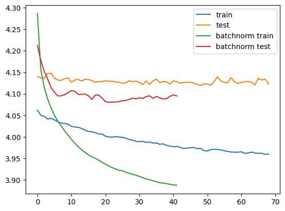
학습 속도면에서 단 11 에포크가 걸렸다.
테스트의 비용함수도 4.119에서 4.080으로 개선되었다.
비교를 위해 모든 그래프를 한 번에 그려보았다.
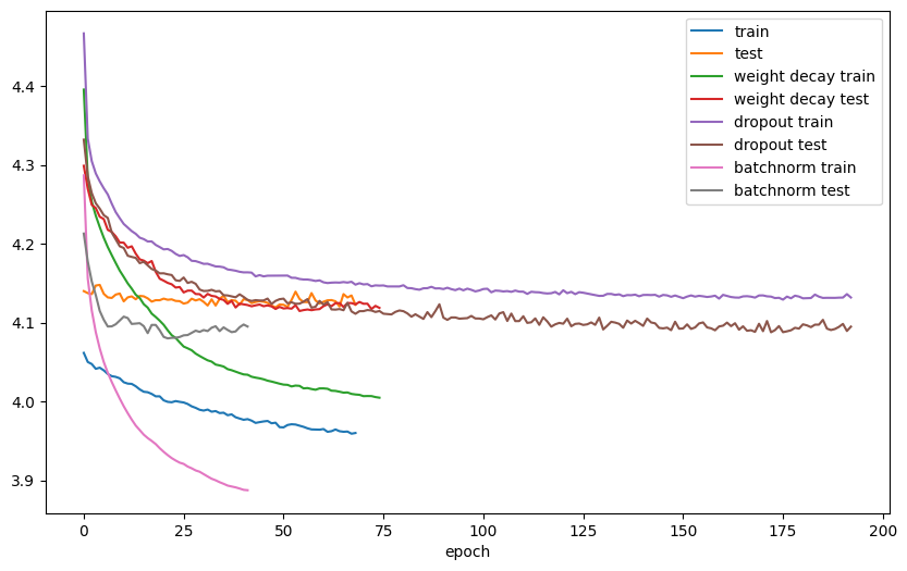
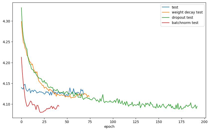
좋고 나쁨을 말하려던 것은 아니었지만 BatchNorm과 Dropout이 실제로 자주 쓰이고 성능도 다른 것들보단 좋은 것을 확인할 수 있다.
사람들이 정규화를 위해 개발한 테크닉은 아주 많다.
우리는 단지 일부분만 다뤘을 뿐이다.
다양한 방법을 시도하여 가장 효과적인 방법을 찾자.